Context
I am presenting an alternative solution to a telecom company to power it’s off-grid towers. The sites are working 24 hours a day, with an average load demand of 2.75 kW.
They are currently running with a DG of 16.2 kW, with an estimation consumption of 11 255 liters. (The consumption estimation is based on a calculation shown in the next chapter).
The site is located in a GCC country.
Assumptions
DG fuel consumption
Based on the provided datasheet of the DG, the fuel consumption is as follows:
| Fuel consumption | l/h |
|---|---|
| Prime power | 5.3 |
| 75% of prime power | 4.0 |
| 50% of prime power | 2.9 |
The estimated lineal curve of the consumption would be:
fuel_c = 4.8 * Gen_c + 0.47
Financial assumptions:
The calculations on the LCOE can be tricky and varies a lot. For this reason, I suggest to read this article.
- DG rental: 745 USD/month.
- Battery price reduction: An advantage when simulating cashflow, is to estimate the new price that the battery will have in the future. I usually choose 1% price reduction per annum. The information that I have been reading lately, is that price expectations as currently is shared among the community is wrong. Moshiel Biton, CEO of Addionics, shared with Energy Storage Report that “argues analysts’ battery price projections are inaccurate”.
- Fuel price: 0.168 USD/l, but I estimated it as 0.17 to include some additional cost of transportation. I assume it is bigger, but we have to accept this amount for now.
- Fuel price increment: 1% per annum. Based on the last developments, this increment is very optimistic.
- O&M system cost: 40 USD/year.
- O&M PV cost: 4 USD/kWp per year. Another value that we must carefully review.
- Discount rate: 6%
- Available battery cycles: 4500 cycles, based on the values from Solar MD’s battery. The specification is showing only that the no of cycles is > 4000.
- Lifetime of the solution: 25 years. Based on the lifecycle of the PV modules.
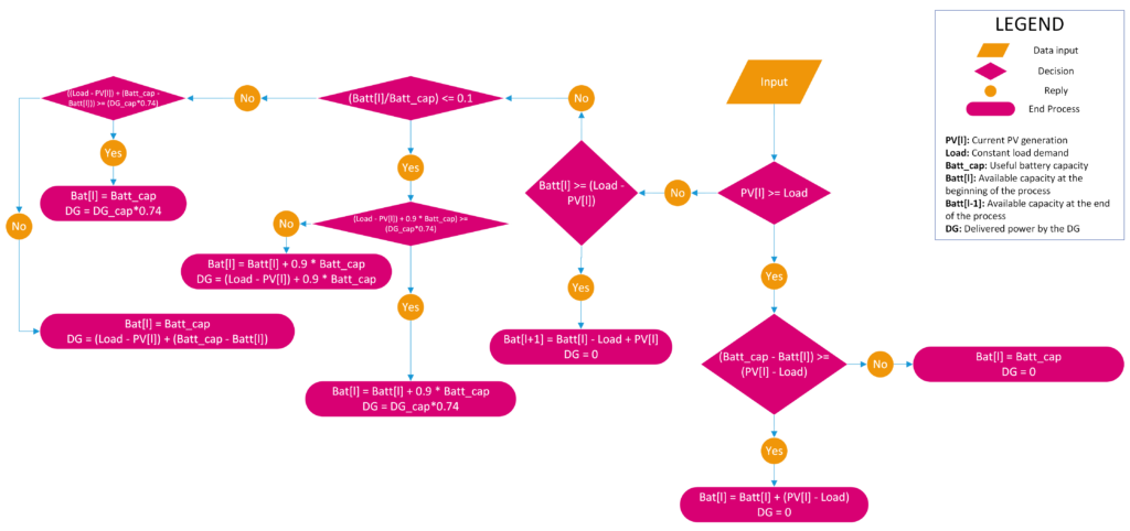
Algorithm
Code
import pandas as pd

gen = pd.read_csv('Gen_site.csv')
PV_basic = gen['P'].to_list() #It is faster to make iterative calculations with lists instead of dataframes
PV_range = 13.2 #Proposed power in kWp
Batt_hours = 16 #Proposed capacity in hours
Load = 2750 #in W
DG_cap = 16200 #in W
PV = [j * PV_range for j in PV_basic] #Comprehension list where I multiply each value of the list times the PV nominal capacity.
Batt_cap = Load * Batt_hours #Battery capacity in Wh
Batt_cap is the full capacity of the battery, and I think there is room for improvement here since the battery should be used only to the 90% of it’s capacity.
Batt = [] #The values of the available battery capacity in each hour will be stored here.
Batt.append(Batt_cap) #The first value at the beginning is of the battery fully charged.
Fuel = [] #The values of the consumed fuel at the end of each hour will be stored here.
DG = [] #The values of the DG output power will be stored here.
logic = [] #This list helps me find which part of the algorithm was applied.
for l in range(0, len(PV)):
    if (PV[l] < Load) & (Batt[l] >= (Load - PV[l])):
        Fuel.append(0)
        Batt.append(Batt[l] - Load + PV[l])
        DG.append(0)
        logic.append(1)
    elif (PV[l] < Load) & (Batt[l] < (Load - PV[l])) & ((Batt[l]/Batt_cap) <= 0.1):
        if ((Load - PV[l]) + 0.9 * Batt_cap) >= (DG_cap*0.74):
            DG_demand = DG_cap*0.74
        else:
            DG_demand = (Load - PV[l]) + 0.9 * Batt_cap
        Fuel.append(4.8 * (DG_demand/DG_cap) + 0.47)
        DG.append(DG_demand)
        Batt.append(Batt[l] + 0.9 * Batt_cap)
        logic.append(2)
    elif (PV[l] < Load) & (Batt[l] < (Load - PV[l])) & ((Batt[l]/Batt_cap) > 0.1):
        if ((Load - PV[l]) + (Batt_cap - Batt[l])) >= (DG_cap*0.74):
            DG_demand = DG_cap*0.74
        else:
            DG_demand = (Load - PV[l]) + (Batt_cap - Batt[l])
        Fuel.append(4.8 * (DG_demand/DG_cap) + 0.47)
        DG.append(DG_demand)
        Batt.append(Batt_cap)
        logic.append(3)
    elif (PV[l] >= Load):
        Fuel.append(0)
        DG.append(0)
        if (Batt_cap - Batt[l]) >= (PV[l] - Load):
            Batt.append(Batt[l] + (PV[l] - Load))
            logic.append(4)
        else:
            Batt.append(Batt_cap)
            logic.append(5)
In each condition of the algorithm I have added a unique value that will help me trace the conditions behind every result. This is the reason of creating a list called logic.
After running all the values of the system in lists, I can now move them back to the dataframe. The reason to do it outside the dataframes is because dfs are designed to fastly apply a specific logic in a whole column. Unfortunately, the values that I create here are depending on previous values. If I use dataframes for this, the time is exponentially slower. That is why this is the fastest way.
Also, the only reason that I continue with dataframes is because they are easier for searching values depending on time. Otherwise, I would only stay with lists. I am saying this because in a later stage, I will have to come back to lists to represent some graphs because I was not able to do it using dataframes.
gen['Fuel'] = Fuel
gen['DG'] = DG
gen['Batt'] = Batt[:-1] #The last value of this list will be the end stage/initial stage of the first hour of the next year.
gen['SoC'] = gen['Batt']*100/Batt_cap  #The multiplication and the Batt_cap division is to create a % SoC.
gen['logic'] = logic
gen['P'] = PV
gen = gen[['time', 'P', 'Fuel', 'DG', 'Batt', 'logic']]
gen['time'] = pd.to_datetime(gen['time'], format = '%Y%m%d:%H%M')
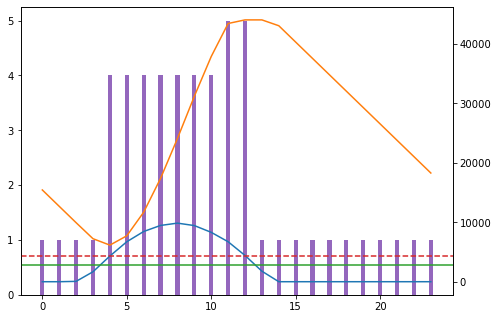
Plotting one day
#Plot a specific day
gen_time = (gen['time'] > '2015-09-02') & (gen['time'] <= '2015-09-03')
import matplotlib.pyplot as plt
X = [i for i in range(len(gen[gen_time]))] #A list with the hours.
Y = gen[gen_time]['P'].to_list()
W = gen[gen_time]['Batt'].to_list()
Z = gen[gen_time]['logic'].to_list()
As mentioned before, I faced issues to integrate in a same figure different graphs, in this case a bar graph with some charts. The available solution was to convert the values into a list and use an object-oriented approach to show the graphs. I believe the main reason was that the two types of graphs created two different type of X-axis that were not compatible, even though it should be the same. X-axis in this case is time.
fig = plt.figure()
ax = fig.add_axes([0,0,1,1]) #Still not sure what is this for. I have copied it from another code I found online.
# Add bar plot
ax.bar(X, Z, color = 'tab:purple', width = 0.25, label='logic')
# Adds line plots
ax2=ax.twinx() # this is the module that solved my issue and I managed to share same X axis with different plots.
ax2.plot(X, Y , color = 'tab:blue', label='P')
ax2.plot(X, W , color = 'tab:orange', label='Batt')
ax2.axhline(y = Load, color = 'tab:green', linestyle = '-') #This line represents the load.
ax2.axhline(y = 0.1*Batt_cap, color = 'tab:red', linestyle = '--') #This line helps me see if the battery has reached the 90% DoD.
For more colors, please check the list here:
List of named colors – Matplotlib 3.5.1 documentation
Calculating the no of cycles
An important value to have in mind while finding the payback or the LCOE, is to know when should we replace the batteries. For now, we know the no of cycles that they can withstand, but we need to know how many cycles is estimated to be used per year.
That is why I created a logic that checks every time the values of the SoC pass from increasing to decreasing..
stat = []
for m in range(1,len(Batt)):
    if Batt[m] > Batt[m-1]:
        stat.append(0)
    else:
        stat.append(1)
cycle = 0
for n in range(1,len(stat)):
    if (stat[n] == 1) & (stat[n-1] == 0):
        cycle += 1
print(cycle)
The result is 734 cycles per year.
Estimating the cashflow and the LCOE
Calculating the LCOE is a formula that needs to be developed separately. Since time was pressing for this specific case, I decided to come back to EXCEL and use the tables I already have for a faster getaway. If you are interested in those tables, please feel free to contact me.
Possible improvements
- To include the derating of the PV modules over time.
- To improve the battery model from a simple lineal battery to a more realistic SoC and SoH model. In addition, SoH can substitute the need of calculating the cycles.
- To implement the LCOE in Python.
For more information, or if you are interested in the most advanced versions of this analysis, feel free to contact me.